5. To count the number of visible rows
Let’s say you are given an Excel table listing all Winter Olympics events, medals, athletes, and countries. The question might arise: “How many gold medals were won by Sweden?”
On the Data ribbon, select Filter. This will put drop-down lists for each column.  Make your selection, by setting two filters in the “Medal”= “gold” and “Country” = “Sweden” columns. (Note: to do this only using the keyboard, use Arrow down to move and Tab to select.)
In the bottom row, type in “=SUBTOTAL(3,A11:A268)”. In this case, the first argument 3 refers to the COUNTA function—a simple count of all alphanumeric characters.
Note that if you typed in “=COUNTA(A11:A268)” the application would ignore the filtering for country/medal that you had just done.
6. Searching with multiple conditions
In the previous example, we had only two non-overlapping filter criteria, Gold and Norway. If we wanted to search for how many gold medals were won by, say, Norway, Sweden, Finland, and Denmark, we would have to use Advanced Filter.
First, insert 6 rows above the table of data. (Zelman called this the “sandbox” and you can think of it as where we play around with the search criteria.) Copy the same headings as the database table.
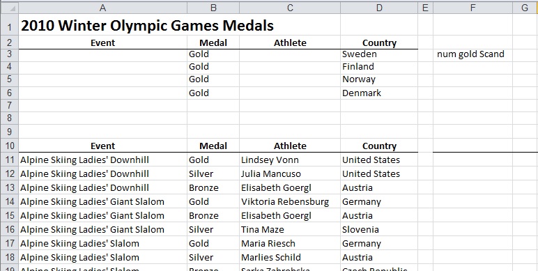
Under the headings, in each row, list Medal = gold and Country = one of the 4 mentioned. The spreadsheet should look like this:
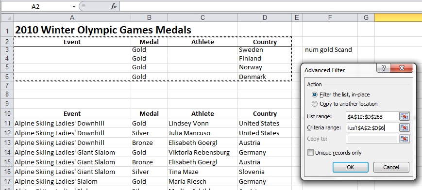
On the Data ribbon, click on the Advanced Filter button. [Or, using shortcut keys, type Alt+A+Q].
In the dialog box that appears, specify the region of the database as the List range—that might be hundreds or even thousands of records. Note that you must include the heading row.
The Criteria range will be smaller. Specify the range to be the 4 lines (and heading) of the search criteria.
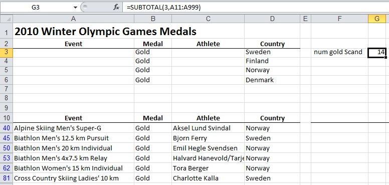
Using the Advanced Filter dialog will show you all rows that fit your search criteria. You can use SUBTOTAL(3,datarange) to help you count the number of visible rows.
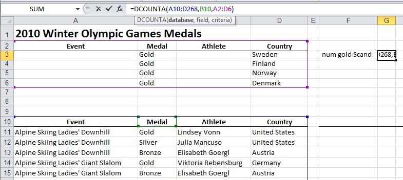
Instead of SUBTOTAL, you can use the DCOUNTA function directly as shown.
A handy trick, no? ª

