
Although Dodd-Frank Act Stress Testing (DFAST) requirements may be the primary motivation for bringing stress testing to the forefront, they should not be the only reason a bank explores the components of loan loss forecasting under a stressed scenario, said Chris Henkel, Senior Director, Enterprise Risk Solutions at Moody’s Analytics. He was the first of two panelists at a webinar held on September 9, 2014, sponsored by the Global Association of Risk Professionals.
An accurate forecast of charge-offs is crucial, Henkel said, so that a firm “can estimate what allowances should be and how large the provisions should be,” thereby predicting the impact on capital reserves. During stressed economic times, such as the most recent financial crisis, “all earnings can be wiped out, due to the provisions” that must be made.
The Federal Reserve Board (Fed) has released a list of some 26 variables that must be stressed for the annual Comprehensive Capital Analysis and Review (CCAR) exercise, first introduced in 2011. However, banks “often consider more variables, if they have externally or internally sourced data” relating to previous financial crises.
Henkel described one approach to modeling Commercial & Industrial (C&I) loan exposures, with the goal of translating a stress scenario to estimated credit losses. The model “divides the large dataset into homogeneous risk pools,” and then develops the relationship for given groups within different sectors (of industry and geography). “We use bootstrapping to ensure continuity.” Model developers looks at R-squared, model robustness, and whether out-of-sample results make sense.
“The starting point for the PD forecast can be an EDF or an internal rating that has been calibrated to a PD,” Henkel noted (PD = probability of default; EDF = estimated default frequency). Better sensitivity to the stressed economic environment is achieved through using point-in-time (PIT) rather than through-the-cycle (TTC) values for model variables.
How do predicted results compare to the actual? Henkel showed graphs of back-testing, and predicted versus actual mean PD for different sectors (such as health care, high tech, and business services); the models achieved good agreement for crisis periods.
 “To translate losses into net charge-offs, the model must explicitly include macroeconomic variables,” Henkel said, and he showed results for forecasting stressed loss given default (LGD) from a commercially available default and recovery database.
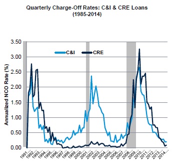
The loss emergence period (LEP), defined as the time from when default occurs until the time when the loss is realized, is another component of the model. On average, over the past two decades, roughly two-thirds of LEPs are less than one year, and one-quarter are from one to two years.
Henkel walked the audience through a simple example of ten firms with LEPs as noted above. The sample firms were low risk, except for three firms with PDs of 0.08, 0.5, and 0.35. The distribution of the loan loss over time was monotonically rising for the 0.08 PD firm, but showed a peak at Q2 for the riskiest firm (PD 0.5). It is instructive to drill down to see what items in the balance sheet give rise to the different time profiles of the net charge-offs. “It has to do with the assumptions around loss emergence,” Henkel explained.
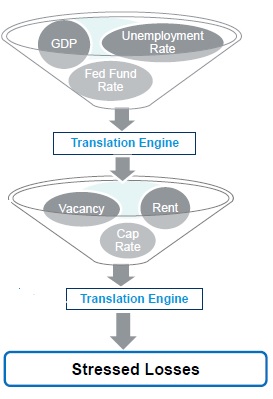
Modeling commercial real estate (CRE) loan exposures was the topic of the second example presented. This combines property forecasting methods with credit risk. The macroeconomic scenario consisting of debt service coverage ratio (DSCR) is the main driver of the default rate; thus, the model must link the economic scenario with the DSCR and the net operating income (NOI). Future values of NOI related to the DSCR are calibrated to historical experience.
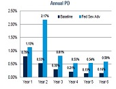
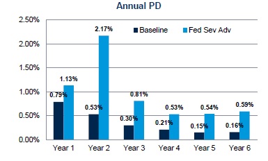
Henkel contrasted a baseline study with the Fed’s 2014 Severely Adverse scenario. He showed how default risk was modeled using different forecast real estate variables while the loan was amortizing in both cases. The Severely Adverse case had default rates peaking in year 2, at about four times the baseline rate. Although default risk subsided in the four years following, the LGD remained high for all four years. The model confirmed experience: that recovery is hard-won. ª
Click here to view the webinar presentation. Chris Henkel’s portion covers slides 5-9 and 14-36.
Click here to read about the second presentation in the Dodd-Frank Stress Testing webinar.