Modelling the economics of an iron ore mine “is a complex task that can be made more reliable,” said David Willingham to a webinar audience on December 5, 2012. Willingham, an application engineer at Mathworks, was demonstrating how a typical mine’s economics could be modelled using MATLAB and then embedded within an Excel spreadsheet.
Developing a mine involves significant capital expenditures and long time frames. Willingham aimed to take the audience through a good model that would take into account the microeconomics of a particular mining company, integrated with the macroeconomic environment, such as interest rates and iron ore prices.
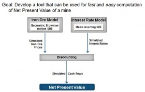
Willingham summarized the overall plan (see schema below) which was to compute the net present value (NPV) of a mine as a combination of two other models: the price of iron ore, and the interest rate at any given time. These are modelled using stochastic differential equations (SDEs) and used to derive the discounting factor that is crucial for calculating the NPV.
Mining forecasts, said Willingham, were an interesting challenge of modelling income vs. costs, uncertainty in prices, and future risks.
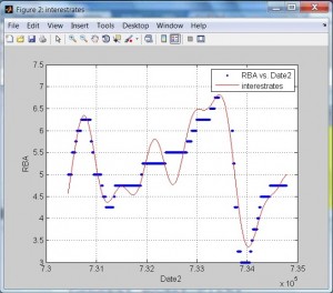
The first task was to model the interest rate. Willingham showed how to fit a curve to interest rate data that were pulled from the Reserve Bank of Australia (RBA) web site. He suggested that it would be most helpful to write an automated script for data import on a regular basis. He chose a sum of sines as the curve fitting model. The real data and the fitted line are shown in the accompanying picture. The overshoots for interpolated points could cause trouble.
Willingham suggested a more sophisticated technique, such as a stochastic differential equation. The mean reverting model of Hull, White, and Vasicek (HWV) assumes a linear regression between the interest rate and its first differences. He said that one thousand simulations of the interest rate could be run in 1.3 seconds.
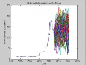
The second task was to model the price of iron ore. Commodity prices are famously volatile. Willingham posed the question: “Will prices stabilize or continue to fall?” He was able to quickly switch between a Vasicek model and a geometric Brownian motion (GBM) model. His example data were in an MS Access database. MATLAB was used to generate SQL commands to fetch the data from indexmundi.com/commodities. A plot of historical and future ore prices is shown below. (History has a single path; the projections of future prices look like a wild assortment.)
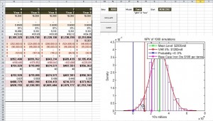
When the two tasks were complete, Willingham used a cash flow script to combine variables such as the production and grade of ore in order to create a histogram of sales. The NPV distribution is shown on the right hand side of the screen shot of the Excel worksheet of Willingham’s presentation.
The NPV distribution analysis shows the mean or expected net present value for that project, and its variance.
Willingham gave a clear and concise walk-through of how to apply MATLAB routines at each step along the way. He showed one instance (curve fitting of interest rates) where an answer could be calculated, but should not be used for other reasons—always an important lesson to modellers. He showed how previous data, in both the interest rate and ore price cases, fed into the stochastic differential equations (SDEs). Results from these gave a discount factor that was needed to estimate the net present value, and thus the economic worth of an iron ore mine. ª
The webinar presentation slides can be found at: http://www.mathworks.com/company/events/webinars/wbnr73971.html?id=73971&p1=1256035947&p2=1256035982
Disclaimer: The author does not hold shares or receive commissions from any products mentioned in this article.

