
“Focus on modelling, not programming,” urged Ameya Deoras, senior applications engineer at MathWorks. He was speaking during a webinar on December 3, 2012 about the use of MATLAB in the construction of financial models.
Deoras’ talk covered four examples to varying depth during the hour. The first example, the calculation of the efficient frontier for large-cap stocks, allowed him to show the easy data importation from an ODBC-compliant database. Each step of the way he showed how the input could be visualized with a single click.
If the data exist in a relational database (think tables and fields such as in SQL), they can be imported through the Visual Query Builder. A Command Window allows direct statements for importing data, or the user can access the data through interactive tools.
“The functions are all designed to work on a matrix of data,” Deoras emphasized. The MATLAB commands are thus compact and uncluttered. For example, “cov(PortfolioA)” will calculate the covariance of the “PortfolioA” matrix of data without your having to write in a single do-while loop. The Visualization key lets you immediately confirm the operation.
Deoras wrote a script to have MATLAB generate a plot of the efficient frontier. He added comment lines that explained the steps as he went “Import Data”; “Calculate Moments”; “Run Portfolio Optimization”; “Create Visualization.” What seemed like standard good coding practice—adding comments—gained new significance when he clicked on the “Publish Script” button and each comment became a heading in a report, and each section contained graphical or tabular output of data, moments, etc.
“You can edit the actual source code of the functions we use,” said Deoras. “This gives validation of the functions—they are not ‘black box’ to the user.” He suggested using source code as a template, if more sophisticated functions are desired [Ed. Note: For example, check out some of the more esoteric risk functions covered in Carl Bacon’s book, Practical Risk-Adjusted Performance Measurement].
The second example Deoras covered concerned econometric modelling, using data pulled from the Federal Reserve Board. He began the model unsure of how many lag orders to use so he fit the auto-regressive model to six different models. For each model he tested the prediction capability—in other words, how accurately each model could predict the econometric measures such as gross domestic product (GDP), unemployment, etc. The default background (white/grey contrast, with grey for the economic downturns) is a helpful feature.
The third example estimated credit risk for a portfolio with 1300 bonds. First, he constructed a one-year N by N transition matrix for N credit ratings based on an internal MATLAB model that uses Z-score. (The model pulls in time series to determine the likelihood of the credit ratings changing.) Once the N by N transition matrix is obtained, it can be used to revalue the portfolio for a Monte Carlo run of, say, 10,000 events. It ran in seconds.
In cases where the code does not run as quickly as expected, Deoras suggested using MATLAB Profiler to determine the time-consuming part of the code that may need attention.
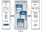
The fourth example concerned the deployment of a MATLAB application in Excel that was based on the first example (portfolio optimization). The developer can create a *.dll, *.bas, or *.xla file that allows other users / clients to run the application, with no need to purchase a separate MATLAB licence for each deployment.
MATLAB does indeed permit the user to focus on modelling, not the minutiae of programming.
ª
The webinar presentation slides can be found at: http://www.mathworks.com/company/events/webinars/index.html?language=en&by=industry&ind=fin
Disclaimer: The author does not hold shares or receive commissions from any products mentioned in this article.