
Let’s say you want to create a predictive model without assuming an analytical form to the model. How would you go about it?
On August 14, 2012, Richard Willey, Technical Marketing Manager at MathWorks, demonstrated via webinar how input data could be fit using machine-learning approaches. The emphasis here is data-driven, as opposed to model-driven, fitting.
“A limitation of regression techniques is that the user must specify a functional form,” said Willey, and the choice of that model is usually based on the domain model. Typically the data points are fit with high-order polynomials or Fourier series. Or, the user might run the data through a library of functions to determine the best fit.
If the user does not want to be locked into a functional form, then statistical learning algorithms such as ‘boosted’ or bagged’ decision trees could be used. These are ensemble methods in which several independent decision trees are created. The weighted average (bagged) or sequential (boosted) forms can be used.
The challenge to any model is that it must be accurate, stable, and generalizable to other datasets. “There is a bias-variance trade-off,” remarked Willey, referring to the likelihood that training on one set of data will tend to make the fit better for that dataset than for any other. A good model will have uncorrelated predictors (and correlated predictors will be easy to identify). It will avoid “overfitting,” where both the trend and the noise are fit. Lastly, the user should be able to calculate the confidence limits of the fit.
Analytic model forms allow estimation of the confidence interval from the least squares fit. When the model is not based on an analytic function, it is still possible to estimate the confidence interval, and Willey showed how that could be done. Briefly, he took N subsets of the data and fit each set. Then he treated the N fits as a population for which he could calculate the confidence interval.
The meat of the presentation was a worked example of data-driven fitting for energy load forecasting. The system load in units of power is some function of time of day, humidity, dewpoint, outdoor temperature, and day of the week. Willey also included lagged variables such as the load of the previous day, and the load of the previous week.
First, he applied the boosted decision-tree method to the dataset. He divided the data into a training set and a test set. He trained, and then he evaluated the fit for accuracy. Central to the work was the method “LSBoost,” short for Least Squares boost, which is a machine learning algorithm.
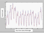
 In that worked example, the biggest predictors, he found, were the two lagged variables named above. The fit and the original data are shown in the accompanying figure. The peaks correspond to evening load, and the troughs correspond to normal sleeping hours. When he presented the distribution of residuals, Willey noted there was a strong pattern for size of residual and the hour of day, therefore, further investigation should be done (beyond the scope of the worked example).
In the following example, Willey re-fit the same energy load dataset with a bagged decision tree method. Examination of the residuals showed that residuals had a much tighter distribution around zero. He concluded that the bagged-tree technique should be used for this type of data. It is difficult to tell a priori whether a boosted or a bagged decision tree technique should be used, so it is recommended to try both.
Willey said that the neural network results gave an even better fit, but the stability was not as good as for a decision tree technique.
When it comes to avoiding model bias, a data-driven fitting technique can be applied. The simplicity of use within the MatLab interface was well demonstrated by this presentation. The code is brief, elegant, and available for download from the MatLab file exchange site. ª
The webinar presentation slides can be found at: http://www.mathworks.com/company/events/webinars/wbnr56627.html?id=56627&p1=961664771&p2=961664789
Product documentation on the Curve Fitting, Statistics, and Neural Networks Toolboxes for the MatLab 11a release can be found at: http://www.mathworks.com/products/examples/