

For generating shocked interest rate curves, such as a sudden economic stress might engender, “a three-factor parameterization solves many problems—but issues remain,” said Alexander Bogin, Senior Economist at the Federal Housing Finance Agency, and the second presenter at a webinar on modelling interest rate shocks held October 28, 2014, and sponsored by the Global Association of Risk Professionals.
To develop an improved yield curve approximation, Bogin showed three variants of non-linear Laguerre functions of time to maturity. These were the Nelson-Siegel model (which has 3 factors); the Svensson model (4 factors); and the Björk-Christensen model (5 factors).
Over a two-year period, Bogin and Doerner used MatLab software to build models for shocks to the interest rate curves. They evaluated their models according to four criteria:
1. Accurate description of observed patterns of yields
2. Flexibility to handle intra-curve constraints (by “intra” they mean within the same curve, for example, a non-negativity constraint)
3. Flexibility to handle inter-curve constraints (by “inter” they mean across different curves, for example, maintaining a plausible credit spread between the Treasury and Libor-Swap curves)
4. Avoidance of negative forward rates
Based on these criteria, they recommend the 5-factor parameterization developed by Björk and Christensen (1999).
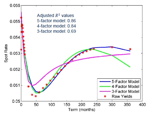
“It’s not as economically intuitive as the 3- or 4-factor model,” said Bogin, “but it gives the closest approximation to historical yield curves and has flexibility in modeling intra- and inter-yield curve constraints.” Also, the Björk and Christensen model can be constrained to non-negative forward rates.
Details on the implementation became apparent when Bogin walked the audience through the six steps of generating historically-based interest rate shocks. The time decay parameter lambda was set to 0.024 throughout. “The model is relatively insensitive to this parameter,” he said.
Bogin began with fitting the market quotes for a LIBOR-Swap spot curve on a particular date, and later repeated the process to simulate agency and Treasury spot curves. If required for stressing the portfolio, they generated “miscellaneous rates” for items such as prime rate, mortgage spreads, and Fannie Mae par coupon.
In the last part of his presentation, Bogin discussed how to generate plausible co-movements in implied volatility. “Implied volatility is a significant risk factor in fixed income portfolios with embedded optionality and a necessary component for a comprehensive shock scenario,” he noted.
Bogin cited several examples of the empirical link between interest rates and implied volatility. For instance, “a sharp decrease in interest rates is often accompanied by increase in implied volatility, such as observed during monetary easing.”
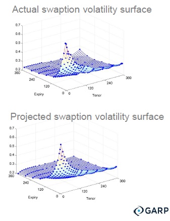
He compared the actual swaption volatility surface with the projected swaption volatility surface, and found the model gave a reasonable fit. ª
Click here to read about the first presentation in the webinar.
Additional details on the work by Doerner and Bogin are provided in FHFA’s Working Paper 13-2 and will be forthcoming in the Journal of Risk Finance.
Click here to view the webinar presentation on modeling stressed interest rates. Bogin’s section covers slides 19 to 45.
We thank the authors for permission to use slides from their presentation.
The photo of the singer Björk is from BBC News Entertainment. No swans were harmed in the creation of this post.