
“Symbolic computing can be a practical part of the solution to your problem,” said Deepak Ramaswamy, technical marketing manager at Mathworks. On January 8, 2013 he showed about three hundred participants via webinar how they could switch between analytical tools in a Notebook app to numerical analysis of the same problem in the MATLAB interface.
He stepped his way through one “classic” and two “real-life” problems: the damped oscillator model; fuel consumption of a rocket-powered car; and kinematics of a double-jointed robot arm. The three problems can be written as systems of Ordinary Differential Equations (ODEs) and this was the starting point for Ramaswamy’s treatment.

There are two ways to access the symbolic math toolbox, he said: via the regular MATLAB interface or through the Notebook app using the MuPAD language. There are over 15 libraries of symbolic math functions available through Notebook, and around 175 Symbolic Toolbox functions available. The Notebook, said Ramaswamy, could be accessed through the Apps Gallery, which is new to MATLAB 2012B.
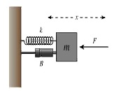
In the Notebook environment, Ramaswamy set up the damped oscillator model as a series of ODEs (in x and t) with initial conditions for x(0) and x’(0). The initial command to “solve” with respect to x gave dense-looking output, so he issued a second command, “simplify” and then recognizable forms appeared. He examined the limit with the critical solution of the equation and showed the simple decaying exponential form that resulted. Given specific parameter values, the software immediately returned positive values to solutions, and these could then be differentiated with respect to time.
When Ramaswamy transferred to the MATLAB window, the equations, although accurate, looked cluttered. The “pretty” command will display formulae in a more digestible form, like a math textbook.
By performing a Laplace transform on the expression, Ramaswamy showed how the poles could be found in seconds—using an analytical approach. Finding the poles numerically would take a minute. Had this been a real-life (i.e. not a tidy model) problem, the difference in time savings could be even more apparent.

“Optimization of the analytic variant is orders of magnitude faster than the numerical variant,” said Ramaswamy. However, he added, “adding fidelity to the symbolic variant can lead to non-solvable systems” that require brute-force numerical solution. He suggested that optimal analytical solutions be used as a starting point for higher fidelity numerical analysis.
The second case Ramaswamy walked through was a real-life model of the Bloodhound Supersonic Car which has a jet, rocket, and two chutes in addition to its car motor (with wheel brakes). All told, there are eight stages of motion as the boosters are fired and then the braking devices kick in. Thus, there are a lot of boundary conditions to set, and ever-changing parameters to account for. Air and wheel surface drag factors are omnipresent.
Ramaswamy showed how the ODEs could be set up and solved for some different stages in order to answer such questions as “when should the rocket be fired and shut off, such that a minimum amount of fuel will be consumed? He called up the Graphical User Interface (GUI) available in the Optimization Toolbox.
The third and final problem concerned inverse kinematics of a two-link manipulator that he constrained to lie in a plane. He solved for the angles of the manipulator and then, to see if the angles made sense, he animated the solution in MuPAD. This was a fast demonstration of how MATLAB could access expressions in Notebook, and how Simulink blocks could be created. ª
The webinar presentation slides can be found at: http://www.mathworks.com/webex/recordings/NA_2013_01_08_numerical_analysis_MATLAB/index.html?s_v1=50274809_1-FSJ9S8
Disclaimer: The author does not hold shares or receive commissions from any products mentioned in this article.