

“One needs to be careful and not over-reliant on any one model,” said Scott L. Smith, Associate Director for Capital Policy at the Federal Housing Finance Agency (FHFA). He was referring to the financial models used by major financial institutions to estimate potential losses. On February 4, 2015, he was presenting a GARP-sponsored webinar on countercyclical stress tests to set capital requirements.
Smith explained how credit risk is measured for mortgages, and described a way to embed stress testing that uses countercyclical concepts. He and colleague Jesse Weiher, Senior Economist at FHFA, performed dynamic stress testing that was adjusted to current economic conditions.
“There are limitations to the current regulatory approaches,” Smith said. Mortgage credit risk models depend on a variety of characteristics that are related to the borrower and the loan itself, such as of FICO and loan-to-value (LTV), respectively. The models include parameters for the macroeconomic scenario such as interest rates, unemployment rates, and (of greatest interest to Smith’s group) local house prices.
The Dodd-Frank Act requires that risk-based capital be determined under countercyclical conditions. The new Basel regulations also require a countercyclical buffer be used in certain situations. The underlying idea is the same: “Countercyclical capital requires sufficient capital before any crisis,” Smith said.
Smith emphasized that analysts should use a “rules-based” or deterministic model, not stochastic (or discretionary). He said that if the model had been stochastic, no-one would have recognized the 2007 financial crisis was occurring until too late.
A suitable model for mortgage credit risk should yield capital requirements for new acquisitions in a realistic fashion, namely, “in full, up front,” and the capital should “increase during credit expansions, and be allowed to fall during downturns as risk exposure declines.”
Gross domestic product (GDP) has had “a very stable trend over the past century,” said Smith, “and housing is a big part of it.” Once the average trend line has been drawn, the trough is defined as how low housing can go below the trend. The bottom of the trough is the lowest point observed in the historical data. He conceded that basing the trough on historical data is “a weak point” in the model but it works well nonetheless.
Figure 1 shows the real housing price index (HPI) for California (blue line), the trend line (red line) and the line joining the troughs (broken red line). The trough line may be thought of as a constant deep economic stress.
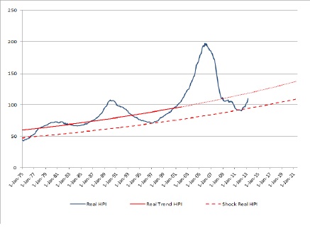
A shock was applied by imposing a path on housing prices from their current level down to the trough. The shock was applied and then released over a specified pattern of years, such as 3 years down to trough, followed by 4 years climbing out of trough. The HPI shock path is done in real terms, then converted to nominal, using inflation rates similar to those in the recent crisis.
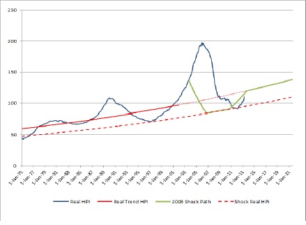
Figure 2 shows a shock that was applied to the HPI line in the year 2003 (green line). Other shock years may be seen in the recording of the GARP webinar around slide 20.ª
Go to Part 2, which describes the second half of the presentation.
All figures shown are used from the webinar presentation with permission from the authors.